Benchmarks
Comparisons against other propagation engines and internal regression benchmarks.
This page reports two sets of benchmarks: comparisons with other open-source Pauli and Majorana propagation engines, and an internal pytest suite for detecting performance regressions.
Results
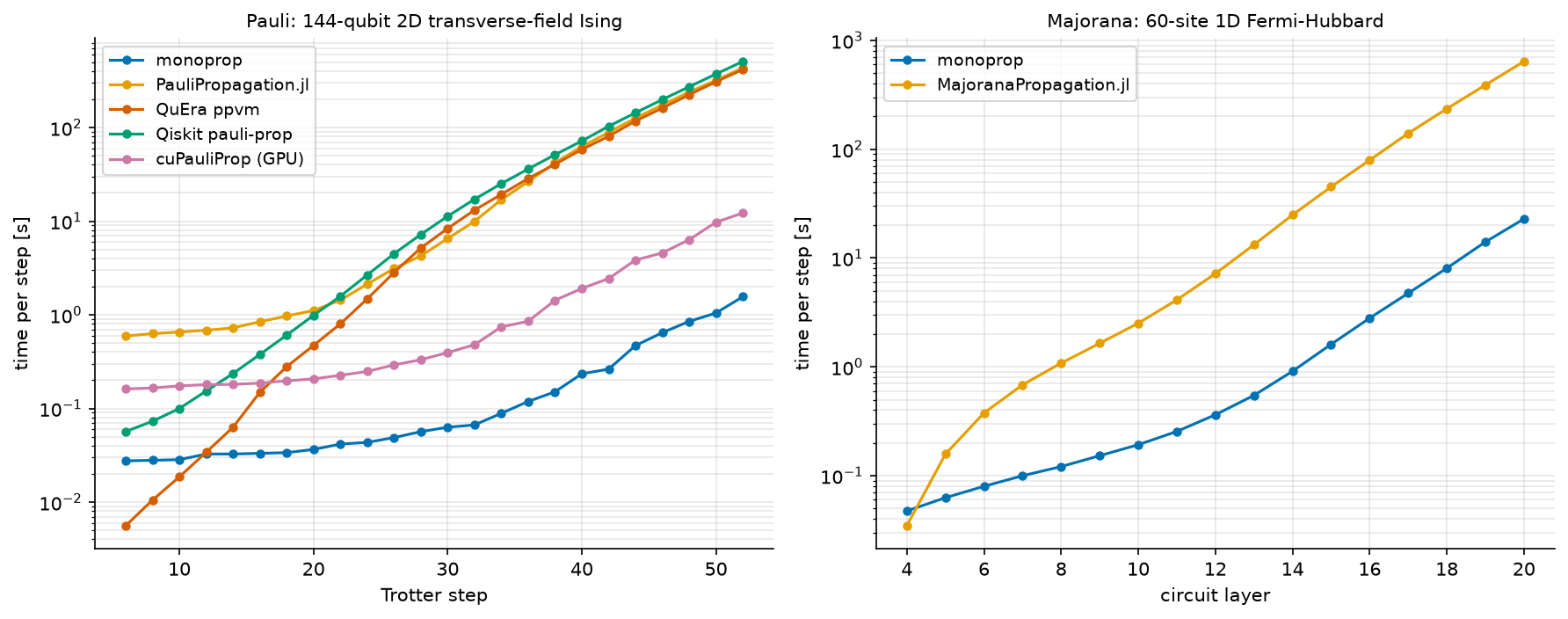
Wall-clock time per propagation step on a logarithmic scale. At the final Pauli step, the
runtime ratios relative to monoprop are 267-325× for the other CPU implementations and 7.8×
for the GPU implementation. Over the complete Majorana evolution, the runtime ratio for
MajoranaPropagation.jl 0.4.1 is 27.7×.
All results were obtained on Leonardo (CINECA); the experimental conditions are specified under Methods.
Pauli propagation
The Pauli benchmark simulates the Trotterized time evolution of a two-dimensional transverse-field
Ising model and evaluates a ZZ correlator on a fixed pair of qubits. One experiment varies the
circuit depth at fixed lattice size; the other varies the lattice size at fixed depth.
Fixed lattice, increasing depth
This experiment uses a 12×12 lattice (144 qubits), 28 Trotter points, dt = 0.05, a coefficient
threshold of 1e-6, and no weight cutoff. The final operator contains approximately 33 million
terms.
| Engine | Final step | VS monoprop | Peak RSS | VS monoprop |
|---|---|---|---|---|
monoprop | 1.56 s | — | 4275 MB | — |
cuPauliProp (GPU) | 12.23 s | 7.8× | 11652 MB (device) | 2.7× |
QuEra ppvm | 417.29 s | 267× | 6956 MB | 1.6× |
PauliPropagation.jl | 433.16 s | 277× | 11102 MB | 2.6× |
Qiskit pauli-prop | 507.74 s | 325× | 34270 MB | 8.0× |
The observables produced by the coefficient-threshold implementations differ by at most 3.8e-4.
Qiskit pauli-prop, which truncates by term count instead, differs by 2.8e-3. The cuPauliProp
operator resides in GPU memory; consequently, the table reports its peak GPU allocation rather
than the host RSS (which we measured at 552 MB).
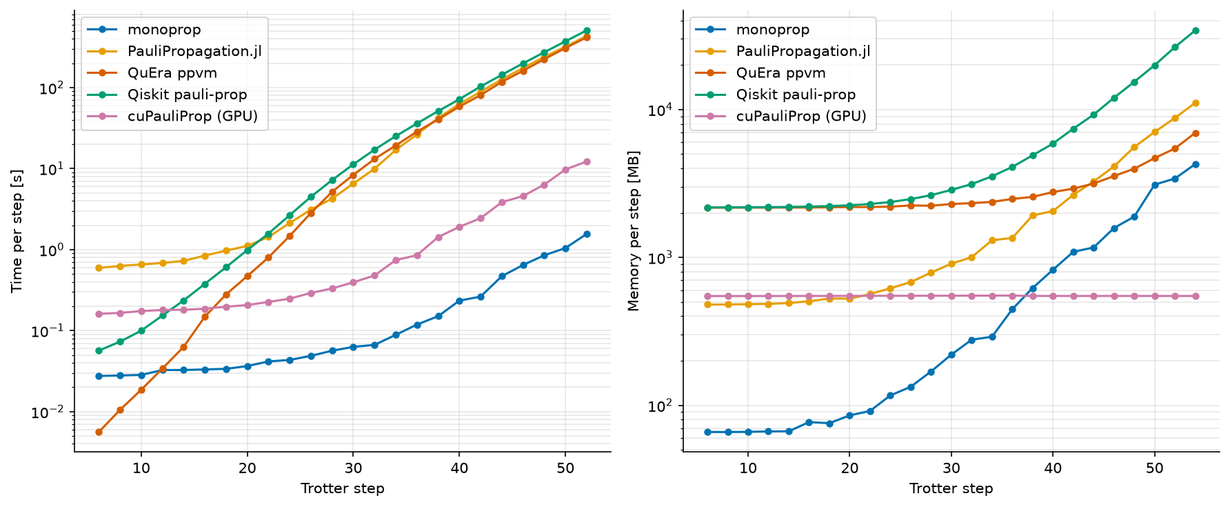
Runtime and peak RSS per Trotter step. Peak RSS is measured by the same procedure for every CPU
implementation; cuPauliProp reports peak GPU allocation.
Increasing lattice size
This experiment holds the circuit depth and truncation threshold fixed while increasing the lattice from 6×6 (36 qubits) to 18×18 (324 qubits). Each model size and implementation runs in a separate subprocess with a 300 s limit.
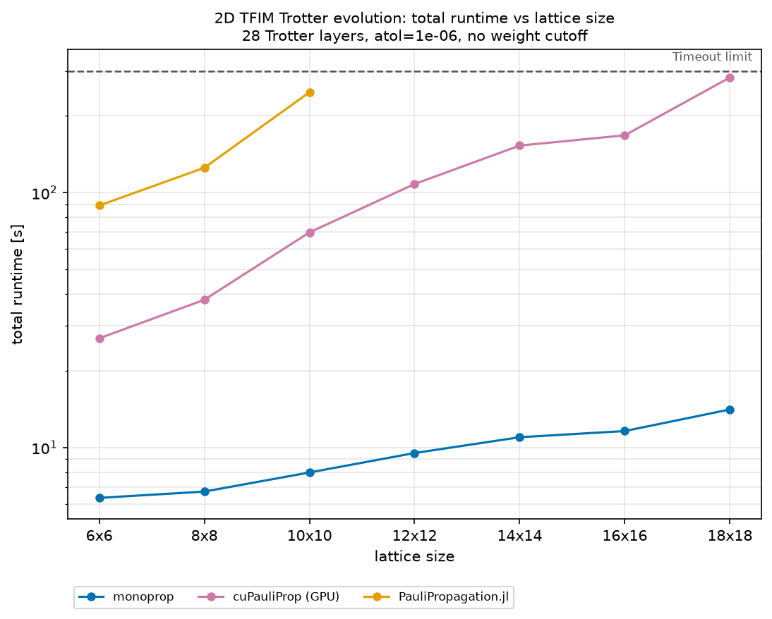
At the selected coefficient threshold, the operator size saturates at approximately 55.0
million terms above 100 qubits. Beyond this point, the experiment primarily measures the cost
per retained term. Across the full range, monoprop runtime increases from 6.35 s to 14.1 s
(2.2×), while the qubit count increases 9×.
The 300 s limit excludes QuEra ppvm and Qiskit pauli-prop at all lattice sizes, and excludes
PauliPropagation.jl above 10×10. We remark that this is not an implementation limit for the packages but a consequence of the timeout limit.
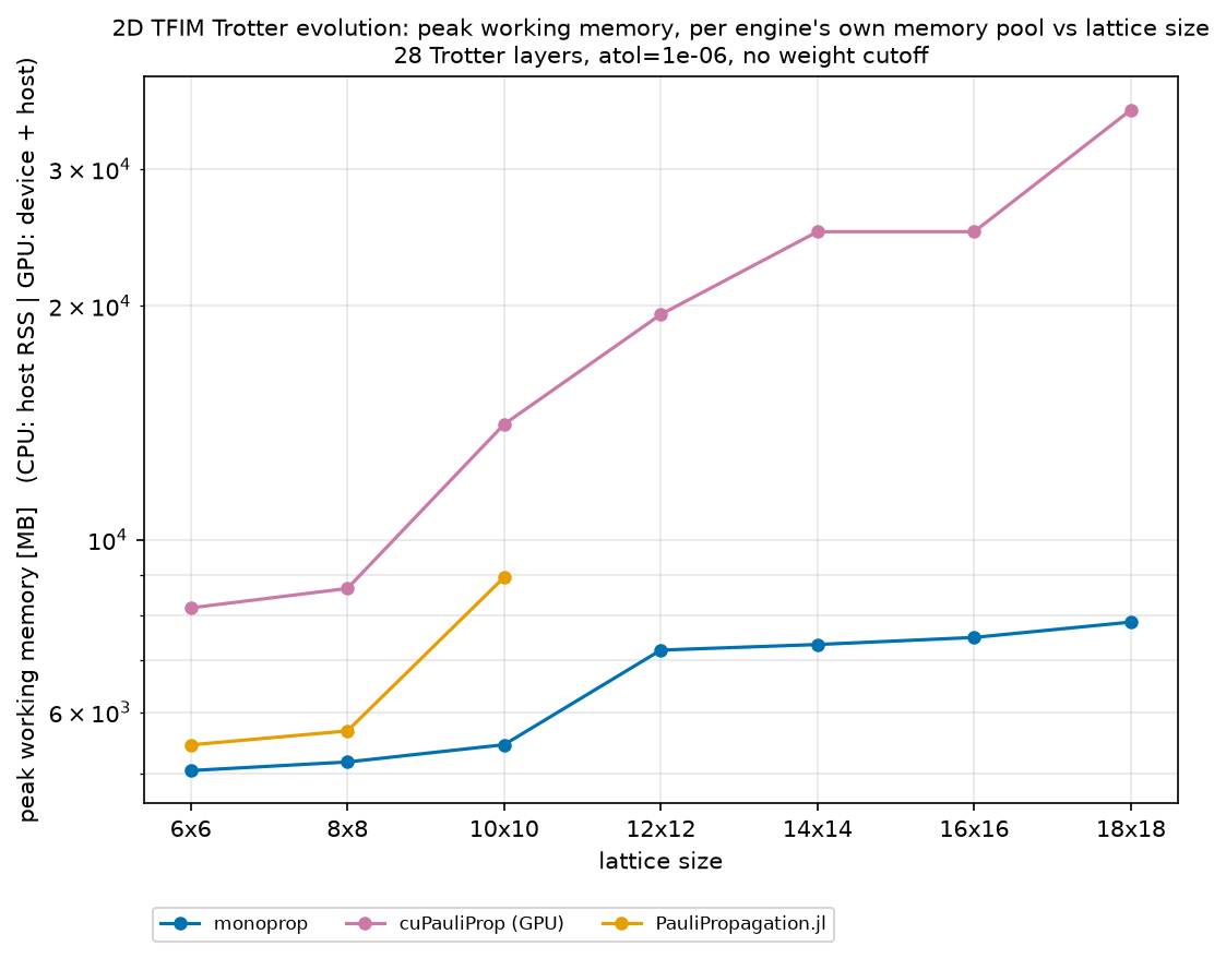
Working memory denotes peak host RSS for CPU implementations and peak device allocation for
cuPauliProp. Across the full range, monoprop increases from 5045 MB to 7835 MB (1.55×),
while cuPauliProp increases from 7.6 GB to 34.4 GB. At 324 qubits, the latter is 4.5× the
monoprop host footprint and occupies more than half of the A100's 64 GB device memory.
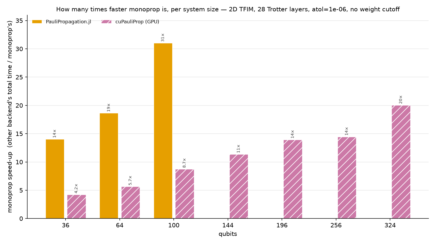
Relative to monoprop, the runtime ratio increases from 14× to 31× for
PauliPropagation.jl over its completed points, and from 4.2× to 20× for cuPauliProp over
the full range. A missing bar denotes a run that exceeded the 300 s limit.
Majorana propagation
The Majorana benchmark simulates 20 Trotter layers of a one-dimensional Fermi-Hubbard model with 60 spinful sites. Runtime, expectation value, term count, and memory are recorded after each layer. Both implementations use 24 threads.
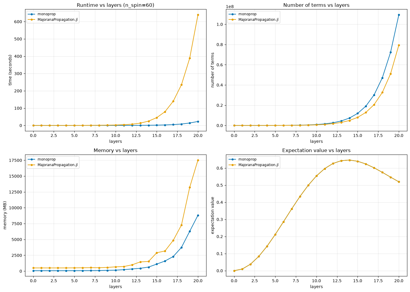
The expectation values differ by at most 2.0e-6 at every layer. At equal truncation,
monoprop retains 109.4 million terms, compared with 79.4 million for
MajoranaPropagation.jl. The complete evolution takes 57.1 s and 1583.7 s, respectively, a
runtime ratio of 27.7×. At the final layer, the corresponding times are 22.9 s and 639.4 s
(27.9×). Peak RSS is 8.8 GB and 17.5 GB, respectively.
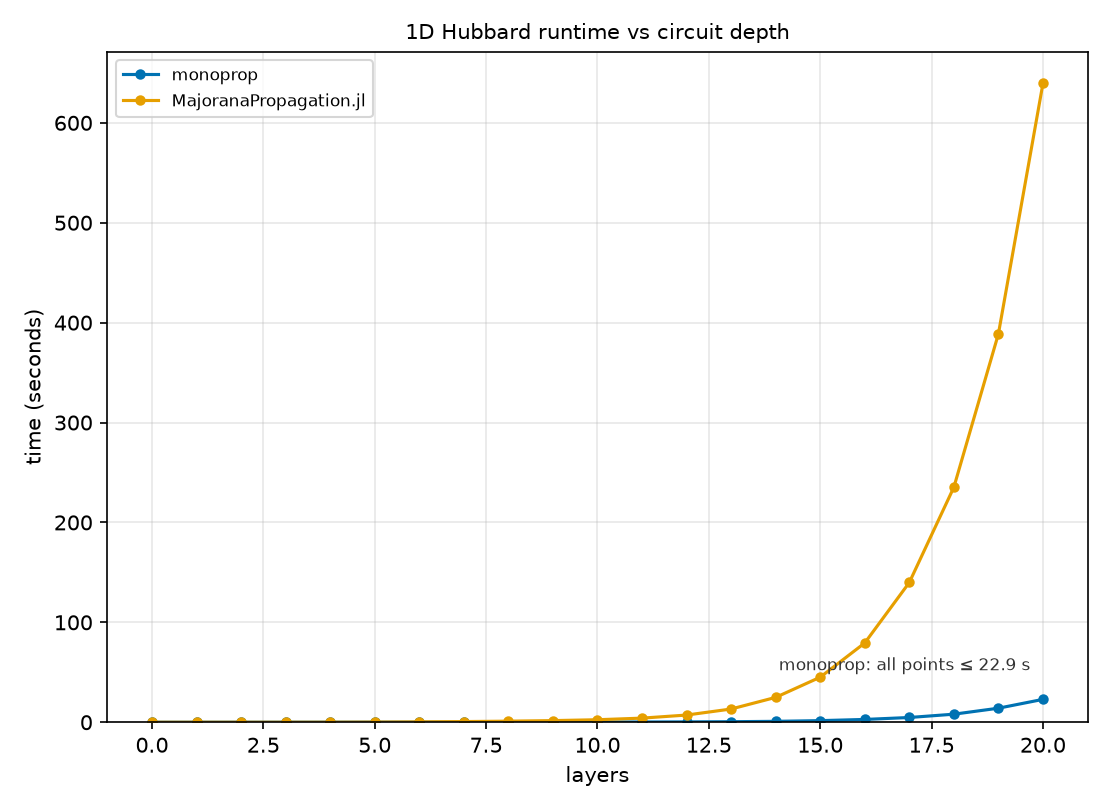
The linear scale preserves the absolute runtime ratio. The annotation gives the upper bound of
the monoprop curve, which otherwise lies close to the horizontal axis.
Caveats
- CPU parallelism differs among implementations.
QuEra ppvmand Qiskit'spauli-propuse one core during propagation (0.99 measured active cores), whereasmonopropandPauliPropagation.jluse multiple cores. TheppvmPython bindings expose the serialindexmapvariant rather than the Rayon-parallelconfig::dashmapvariant; Qiskit's_accelerateextension has no parallel propagation path. Runtime ratios are therefore wall-clock ratios, not per-core ratios. - The Julia benchmarks use the fastest documented containers. These are
VectorPauliSumwithPerformance.propagate!(development branch 0.8.0 or later) andVectorMajoranaSumwith AcceleratedKernels. Their dictionary-backed alternatives are serial. The vector Pauli path does not merge duplicate strings, so its reported term count is a storage count rather than the number of distinct operator terms. - The CPU and GPU measurements use different node types. Each scaling curve is obtained on a
single node. The
cuPauliPropruntime comparison nevertheless includes both hardware and implementation effects.
Methods
The benchmark drivers are maintained in
packages/bench-third-party,
a standalone uv project with its own lockfile. It is excluded from the repository workspace
because it requires CUDA-specific wheels and a narrower Python version range than monoprop.
Hardware
The measurements use exclusive nodes on Leonardo (CINECA). CPU and GPU measurements use different partitions because Leonardo's DCGP nodes do not contain GPUs.
| Partition | Hardware | Engines |
|---|---|---|
| DCGP (CPU) | 2× Intel Xeon Platinum 8480+, 112 cores, ~480 GB RAM | monoprop 0.8.1.dev61+gcb9a033aa (56 threads), PauliPropagation.jl 0.8.2 on Julia 1.12.6 (28 threads), QuEra ppvm 0.1.0, Qiskit pauli-prop 0.2.0 |
| Booster (GPU) | NVIDIA A100-SXM-64GB, 8 host cores | cuPauliProp via cuquantum-python-cu12 26.6.0 |
The benchmarks use each engine's best known configuration. monoprop uses all 56 cores of one
socket; PauliPropagation.jl uses 28 threads because higher thread counts reduce its throughput.
Each result record includes host, threads, and library_version; the plotting scripts report
these fields alongside derived metrics.
How memory is measured
CPU memory denotes peak resident set size (RSS), obtained from the Linux kernel's VmHWM
counter. RSS is the physical memory resident for one process; pages shared with other processes
are counted in full. For cuPauliProp, whose operator resides on the GPU, working memory
instead denotes peak device allocation.
- The measurement is exact. The kernel updates
VmHWMwhenever RSS increases, including during native code that does not hold the Python GIL. - The measurement interval is reset for each step. Before resetting
VmHWM, the harness runsgc.collect()andmalloc_trimfor Python, orGC.gc()andmalloc_trimfor Julia. The resulting value excludes peaks retained from earlier steps. - All CPU implementations use the same measurement procedure over the timed region.
RSS includes the interpreter and loaded libraries. Comparisons of growth across steps therefore carry less fixed overhead than comparisons of absolute values.
Implementation-specific estimates are also recorded as native_memory: operator_memory_bytes()
for monoprop, Base.summarysize for PauliPropagation.jl, and device-pool usage for
cuPauliProp. These estimates cover different allocations and are therefore suitable only for
comparison within a single implementation.
Reproducing
The Python implementations share one uv environment:
cd packages/bench-third-party
uv sync    # monoprop (editable), qiskit, ppvm, pauli-prop, cuquantum-python-cu12
Julia is required only for the Julia comparisons:
curl -fsSL https://install.julialang.org | sh          # juliaup + latest stable Julia
julia -e 'using Pkg; Pkg.add(["JSON", "ProgressMeter"])'
The benchmark and plotting commands are:
# Pauli, fixed lattice; edit settings.json to change the model
cd pauli_prop
uv run python run_model.py        # CPU engines -> results.json
julia run_model.jl                # optional; merges PauliPropagation.jl in
uv run python run_model.py --backends cupauliprop -o results_gpu.json   # on a GPU node
uv run python plot_results.py

# Pauli, lattice sweep; 300 s limit per (size, engine)
uv run python run_scaling.py --output scaling_cpu.jsonl --timeout 300 \
    --backends monoprop juliapp ppvm qiskit --threads monoprop=56 juliapp=28
uv run python run_scaling.py --output scaling_gpu.jsonl --timeout 300 \
    --backends cupauliprop                                   # on a GPU node

# The first input takes precedence when a backend occurs in both files
uv run python plot_scaling.py scaling_cpu.jsonl scaling_gpu.jsonl
uv run python plot_scaling.py scaling_cpu.jsonl scaling_gpu.jsonl \
    --memory-key working_set_MB
uv run python plot_speedup.py scaling_cpu.jsonl scaling_gpu.jsonl

# Majorana
cd ../majorana_prop
monoprop_NUM_THREADS=24 JULIA_NUM_THREADS=24 bash run_benchmarks.sh

# Two-panel headline figure from both committed result sets
cd .. && uv run python plot_headline.py
CPU and GPU scaling results are stored separately and combined during plotting. If an
implementation occurs in more than one input, the first input takes precedence; placing the CPU
file first ensures that the monoprop curve contains only CPU-node measurements.
plot_scaling.py warns when a curve contains multiple hosts and does not label an axis as host RSS
unless all included records use that metric.
All Pauli model parameters are defined in
settings.json
and are shared by all implementations. Output schemas, field definitions, and implementation-specific
limitations are documented in
packages/bench-third-party/README.md.
Internal benchmarks
The internal pytest benchmark suite measures the runtime and peak RSS of core monoprop
operations. It is separate from the functional test suite and runs with just bench.
Running
Each run requires a label, which identifies its column in results/REPORT.md. This permits
direct comparison of serial, threaded, and MPI configurations. Additional arguments are forwarded
to pytest.
uv sync --group bench                          # once

just bench serial                              # serial run, column "serial"
just bench-smoke                               # quick sanity check (tiny sizes)
just bench serial --num-modes 64 --bench-rounds 10

monoprop_NUM_THREADS=10 just bench serial-t10  # cap the partition count

uv run --group bench monoprop-bench-report benches/results  # rebuild report, no re-run
Both groups measure the same four operations -- build_graph, propagate, energy and
gradient -- so a number means the same thing whichever problem produced it:
bench_random.pyruns them on a random problem, in both the Heisenberg and the Schrödinger picture. Configurable with--gen-length(4),--obs-terms(10000),--num-generators(100),--num-modes(128),--cutoff(6),--seed(0) and--bench-rounds(1); defaults in parentheses.bench_models.pyruns them on two fixed models markedslow, Heisenberg only: a 120-qubit Fermi-Hubbard 29-step Trotter run ([hubbard]) and a 127-qubit kicked-Ising run over 20 layers ([pauli]). Override any config field with--<model>-<field>, e.g.--pauli-num-layers 30;just bench --helplists them all.
Run one group per process at scale: build_graph/propagate and energy/gradient each hold
their own operator, and running all four together holds two per rank.
Each run writes pytest-benchmark timings to results/time-<label>.json and the remaining metrics
to <label>.json. monoprop-bench-report combines all labels in results/REPORT.md.
MPI
For MPI benchmarks, barriers delimit each timed operation; runtime is therefore the makespan across ranks. Memory is the sum of the per-rank peak RSS values. This is an upper bound on the job-wide peak: shared pages are counted once per rank, and rank-local peaks are summed even when they occur at different times.
just bench-build-mpi                           # build once (MPI on)
monoprop_NUM_THREADS=2 just bench-mpi r5t2 5 --map-by slot:PE=2 --bind-to core
Rungs
The default sizes above fit a laptop and a CI runner. The sizes the library is actually used at
do not, and a benchmark set that exists only as flags in someone's shell script cannot be
reviewed, reproduced or compared across campaigns. benches/rungs.toml is therefore the
benchmark set itself: one row per cell, giving the picture, the model, the operations, the
geometry, the size knobs, and the exact term count that configuration is known to produce.
monoprop-bench-rung benches/rungs.toml list                        # the whole set
monoprop-bench-rung benches/rungs.toml <id> --dry-run              # the plan, no allocation
monoprop-bench-rung benches/rungs.toml <id> --rep 3 --results runs # one rep
monoprop-bench-ladder benches/rungs.toml runs                      # the block to paste
Nothing runs these for you. They are the fixed benchmark set; running the ones a change could
plausibly move, and putting the result in the pull request, is the author's job. That is what
monoprop-bench-ladder prints: the timings, the peak memory, and the resolved parameters of every
problem measured -- read back from the run rather than from the row's overrides, so a reviewer can
see what was measured without resolving flags against a model's defaults.
Each row also declares cost_seconds and cost_gib_per_node: what one rep last cost, so you can
see what a rung will take before you spend it, and so the collated table can show this run against
the last one. Those two are documentation, never a gate -- a timing is noisy and your machine is
not the machine they were taken on.
A rung declares expect_terms, and a result that misses it by more than 0.1% is refused: the
term count is reproducible to the digit at a fixed seed and tolerance, so a mistyped knob then
fails the cell instead of quietly measuring a different problem. The runner checks the geometry it
actually ran under the same way, and refuses a run with more than one timing round, because
pedantic builds round k+1's arguments before releasing round k's -- two propagators are
resident at once and peak memory doubles. Repetition comes from repeated invocations, which is
what --rep names.
A row nobody has calibrated refuses to run at all. It says so twice: expect_terms = 0, and
TBD in place of any size knob still to be measured. The knob is spelled TBD rather than left
at 0 because 0 is not neutral -- lower_atol = 0 prunes nothing and is the largest problem
the model can pose, so a placeholder 0 invites exactly the allocation-burning run the gate
exists to prevent.
Sizes come from the coefficient tolerance, not from the cutoff or the system size: at the default
lower_atol = 1e-4 both fixed models are saturated in both, so a sweep over either measures
nothing.
Every operation runs the same 10M / 100M / 1B / multinode-1B ladder, and some of the graph rungs
may not fit. build_graph extends the graph rather than replacing it, so it retains one
layer-set per gate while propagate releases each layer as it contracts -- Hubbard reaches 97M
terms in well under 2 GiB through propagate, while four successive build_graph calls on the
same model exceed a 242 GiB node, and at 1000 generators the retained layer count is an order of
magnitude larger again. Which of the graph rungs fit is therefore a question calibration answers,
not one the table should pre-empt: a row that does not fit records the node count it needed, or
that it exceeded the machine, and stays uncalibrated. That is itself a measurement of what the
graph path costs.
Running a rung needs a machine, a scheduler and an allocation, none of which belong in this repository. The table, the runner and the gate are here; the launcher that submits them is not.
benches/RUNGS.md is the operator's guide: every model's parameters and what they do, how the
geometry maps onto a machine, example Slurm scripts, the pinning and allocation-sizing traps, and
how to calibrate a row nobody has measured.
Scaling
Node scaling of Hubbard propagate in the shipped default configuration, 1 to 64 nodes (128 to
8192 cores) at 8 MPI ranks per node × 16 partitions, so R = 8N and P = 128N with one core per
partition. Measured 2026-08-27 on AMD EPYC 7742 nodes with 242.0 GiB usable each; 38 rungs, five
reps apiece (ten on the smallest weak ladder), every rep gate-checked on binary identity,
environment and term count before its time was kept. These rungs are rows in rungs.toml; the
medians below are the cost_seconds and cost_gib_per_node those rungs declare.
Problem size is --hubbard-lower-atol at a fixed cutoff of 10, which is saturated there, so all
growth comes from the tolerance and every rung stays inside the same operator family. The eleven
sizes form a doubling sequence and both families are built from it, so a cell reached by two
ladders is exactly the same problem — nine such cells agreed to within 1.24%, most within 0.2%,
which is a free check on the whole apparatus.
Some rungs are absent because the problem does not fit in that many nodes' memory, not because
they were skipped: strong-6126m starts at two nodes and strong-24420m at eight.
strong-1569m — 1,569,152,761 terms held fixed.
| nodes | R | P | terms | Mterms/node | median s | Mterms/s/node | GiB/node |
|---|---|---|---|---|---|---|---|
| 1 | 8 | 128 | 1,569,152,761 | 1569 | 215.61 | 7.28 | 99.9 |
| 2 | 16 | 256 | 1,569,152,761 | 785 | 105.91 | 7.41 | 51.5 |
| 4 | 32 | 512 | 1,569,152,761 | 392 | 53.34 | 7.35 | 28.0 |
| 8 | 64 | 1024 | 1,569,152,761 | 196 | 28.58 | 6.86 | 15.9 |
| 16 | 128 | 2048 | 1,569,152,761 | 98 | 18.12 | 5.41 | 11.0 |
| 32 | 256 | 4096 | 1,569,152,761 | 49 | 16.13 | 3.04 | 6.6 |
| 64 | 512 | 8192 | 1,569,152,761 | 25 | 23.99 | 1.02 | 4.1 |
strong-6126m — 6,125,805,627 terms held fixed.
| nodes | R | P | terms | Mterms/node | median s | Mterms/s/node | GiB/node |
|---|---|---|---|---|---|---|---|
| 2 | 16 | 256 | 6,125,805,627 | 3063 | 450.19 | 6.80 | 200.2 |
| 4 | 32 | 512 | 6,125,805,627 | 1531 | 224.45 | 6.82 | 101.3 |
| 8 | 64 | 1024 | 6,125,805,627 | 766 | 109.53 | 6.99 | 51.3 |
| 16 | 128 | 2048 | 6,125,805,627 | 383 | 58.75 | 6.52 | 27.4 |
| 32 | 256 | 4096 | 6,125,805,627 | 191 | 38.09 | 5.03 | 16.1 |
| 64 | 512 | 8192 | 6,125,805,627 | 96 | 36.95 | 2.59 | 11.4 |
strong-24420m — 24,419,998,198 terms held fixed.
| nodes | R | P | terms | Mterms/node | median s | Mterms/s/node | GiB/node |
|---|---|---|---|---|---|---|---|
| 8 | 64 | 1024 | 24,419,998,198 | 3052 | 471.03 | 6.48 | 201.3 |
| 16 | 128 | 2048 | 24,419,998,198 | 1526 | 235.19 | 6.49 | 101.8 |
| 32 | 256 | 4096 | 24,419,998,198 | 763 | 127.10 | 6.00 | 52.2 |
| 64 | 512 | 8192 | 24,419,998,198 | 382 | 79.58 | 4.79 | 26.9 |
weak-97m — ~97M terms per node.
| nodes | R | P | terms | Mterms/node | median s | Mterms/s/node | GiB/node |
|---|---|---|---|---|---|---|---|
| 1 | 8 | 128 | 96,981,051 | 97 | 10.75 | 9.02 | 10.8 |
| 2 | 16 | 256 | 184,124,520 | 92 | 10.58 | 8.70 | 9.6 |
| 4 | 32 | 512 | 377,482,074 | 94 | 13.13 | 7.19 | 11.5 |
| 8 | 64 | 1024 | 781,669,404 | 98 | 14.54 | 6.72 | 10.9 |
| 16 | 128 | 2048 | 1,569,152,761 | 98 | 18.11 | 5.42 | 11.0 |
| 32 | 256 | 4096 | 3,104,527,573 | 97 | 24.39 | 3.98 | 11.0 |
| 64 | 512 | 8192 | 6,125,805,627 | 96 | 36.59 | 2.62 | 11.4 |
weak-385m — ~385M terms per node.
| nodes | R | P | terms | Mterms/node | median s | Mterms/s/node | GiB/node |
|---|---|---|---|---|---|---|---|
| 1 | 8 | 128 | 377,482,074 | 377 | 47.71 | 7.91 | 26.6 |
| 2 | 16 | 256 | 781,669,404 | 391 | 50.90 | 7.68 | 28.0 |
| 4 | 32 | 512 | 1,569,152,761 | 392 | 53.29 | 7.36 | 27.9 |
| 8 | 64 | 1024 | 3,104,527,573 | 388 | 54.73 | 7.09 | 27.5 |
| 16 | 128 | 2048 | 6,125,805,627 | 383 | 58.03 | 6.60 | 27.4 |
| 32 | 256 | 4096 | 12,255,330,837 | 383 | 64.64 | 5.92 | 26.3 |
| 64 | 512 | 8192 | 24,419,998,198 | 382 | 79.89 | 4.78 | 26.9 |
weak-1529m — ~1529M terms per node.
| nodes | R | P | terms | Mterms/node | median s | Mterms/s/node | GiB/node |
|---|---|---|---|---|---|---|---|
| 1 | 8 | 128 | 1,569,152,761 | 1569 | 215.61 | 7.28 | 99.9 |
| 2 | 16 | 256 | 3,104,527,573 | 1552 | 222.27 | 6.98 | 100.2 |
| 4 | 32 | 512 | 6,125,805,627 | 1531 | 224.04 | 6.84 | 101.2 |
| 8 | 64 | 1024 | 12,255,330,837 | 1532 | 227.33 | 6.74 | 99.9 |
| 16 | 128 | 2048 | 24,419,998,198 | 1526 | 235.55 | 6.48 | 101.8 |
| 32 | 256 | 4096 | 48,317,129,677 | 1510 | 249.62 | 6.05 | 101.3 |
| 64 | 512 | 8192 | 94,684,031,363 | 1479 | 257.05 | 5.76 | 84.3 |
Two things follow from the strong curves, and only from having three of them. The reversal in
strong-1569m at 64 nodes is not a property of a core count: the same hardware still improves at
64 nodes on the two larger problems. What sets the optimum is the load per node, and it falls
below roughly 50–100 Mterms/node at the point each curve turns. Each doubling of the problem buys
one more useful doubling of nodes.
Weak scaling says the same thing from the other side. At ~97M terms/node, 64 nodes runs at 29% of one node's efficiency; at ~385M it is 60%; at ~1529M it is 84% across 64× the hardware. A run that can afford about 1.5e9 terms per node weak-scales almost ideally to 8192 cores; one at 100M/node does not.
Peak resident memory over all 38 rungs, spanning 25 to 3063 Mterms per node:
GiB/node = 3.39 + 0.0634 × Mterms/nodeBoth terms are real. The slope is the per-term cost, about 68 bytes per term. The constant is a
genuine per-node floor that a model through the origin cannot reproduce — the smallest rung
measures 4.1 GiB/node at 25 Mterms/node. Every rung falls within −2.9 to +4.5 GiB/node of that
line except weak-1529m at 64 nodes, which measures 84.3 against 97.1 predicted, identically on
all five reps; it is reproducible and unexplained, and no mechanism is claimed for it on the
strength of one rung. The largest cell measured 201.3 GiB/node against a 242.0 GiB grant.
Continuous benchmarking
The bench_main.yml workflow benchmarks every commit on main. Bencher
records the time series and reports threshold violations. The workflow invokes the same recipes
available locally:
just bench-ci ci-linux          # default sizes, more rounds, no slow models
just bench-bmf ci-linux         # the same results as Bencher Metric Format JSON
monoprop-bench-bmf combines both artifacts because each Bencher upload accepts one adapter. The
standard python_pytest adapter includes timings but omits memory and operator metrics. Three
measures are recorded:
| Measure | Unit | Source | Threshold |
|---|---|---|---|
latency | nanoseconds | pytest-benchmark mean ± 1σ | Student's t-test, upper 0.99 |
peak-memory | bytes | per-operation peak RSS (VmHWM), summed over ranks | +10% |
terms | count | terms in the evolved operator | any change |
For a fixed seed and problem size, terms is deterministic; any change therefore indicates an
algorithmic change. It is tracked for that reason alone: it is the only check that a timing win is
not an accuracy change. Timing alerts from shared runners are recorded but do not fail the build.
latency is the mean, because Bencher's t-test threshold consumes a mean and a spread. A rung
ladder reads the same runs on the median and the min instead -- these distributions are skewed, so
a mean tracks stragglers rather than the cost of the work. The two statistics answer different
questions and neither substitutes for the other.
Testbeds
Bencher identifies each series by (branch, testbed, measure). A testbed therefore denotes one
fixed machine configuration; changing that configuration would introduce a discontinuity in every
series.
| Workflow | Runner | Testbed | Label | Profile |
|---|---|---|---|---|
bench_main.yml | GitHub-hosted ubuntu-26.04 | ubuntu-26.04 | ci-linux | not slow, 5 rounds |
bench_bare_metal.yml | RunsOn EC2 node | aws-c7i-4xlarge | ci-bare-metal | everything, 3 rounds |
The bare-metal workflow provisions a dedicated node for each run. Its lower measurement variance supports tighter timing thresholds and permits execution of the fixed models omitted on the shared runner.
No benchmark workflow gates a pull request. Both track the main branch, and a threshold over a
series that spans runners is a report, not a verdict. Measuring a change is the author's job: run
the rungs the change could plausibly move and put the numbers in the pull request. Rungs above
says how.
The bare-metal workflow is inert until a maintainer sets the BENCH_BARE_METAL repository
variable -- without a RunsOn stack behind the bench label the job would queue until it timed out.
Every run uploads bmf.json and the raw result JSON as an artifact, so a failed Bencher upload
does not take the measurement with it.
The bench-markers and bench-rounds inputs of the reusable bench.yml workflow select the
benchmarks and repetition count. These values should remain fixed after establishing a testbed,
because changing them changes the meaning of its time series:
monoprop_BENCH_MARKERS= monoprop_BENCH_ROUNDS=3 just bench-ci ci-bare-metal